
Interval Width Fuzzy Aggregation for Streaming Process Monitoring on the Tennessee Eastman
Abstract
This study evaluates a transparent interval-width fuzzy anomaly score for streaming process monitoring. The reported IT2-DRA configuration converts standardized variables into Gaussian normality memberships with widths in [0.8, 1.2], takes complementary anomaly memberships, averages their interval endpoints with fixed normalized weights, and smooths the result. The width band is a design assumption; the resulting score is neither an estimated accident probability nor a calibrated measure of epistemic confidence. On 21 classic Tennessee Eastman (TE) fault streams, the reported mean area under the receiver operating characteristic curve (AUC) was 0.8099 ± 0.1667 and the capped detection-delay mean was 251.4 samples. Hotelling T², Multivariate Exponentially Weighted Moving Average (MEWMA), and a shallow autoencoder achieved mean AUCs of 0.9183, 0.9117, and 0.8758 and shorter mean delays. The reported Friedman AUC test gave p = 6.83e−06; Holm-adjusted paired comparisons favored these three baselines. The type-1 counterpart had a statistically detectable but small mean AUC advantage of 0.0006. The false-alarm comparison did not reject equality (p = 0.2483), which does not establish equivalence. A per-variable contribution bound explains why weighted averaging can dilute localized deviations, while joint dependence is not represented explicitly. The findings delimit this interval-midpoint construction on the stated benchmark and do not assess general rule-based interval type-2 inference.
Keywords:Interval-valued fuzzy membershipsAnomaly aggregationTennessee Eastman processfault
Detection, Streaming monitoring, Benchmark comparison.
1. Introduction
Failure Mode and Effects Analysis (FMEA) organizes failure modes by severity, occurrence, and detectability. Fuzzy set theory provides graded memberships [1], and interval type-2 fuzzy sets represent uncertainty in primary memberships through a footprint of uncertainty [2], [3]. Recent applications include interval type-2 FMEA with multiple-criteria decision making [4] and fuzzy risk assessment in the steel industry [5]. These constructions motivate examining how interval-valued memberships behave in a streaming monitoring task; they do not by themselves establish detection performance or safety-risk calibration.
Real-time process safety research connects monitoring with decision support [6]. The Tennessee Eastman (TE) simulation provides a widely used benchmark for evaluating process monitoring [7–9]. The present question is specific: Does a fixed uncertainty band on Gaussian membership widths improve a weighted streaming anomaly score relative to its type-1 counterpart and to multivariate monitoring baselines?
We evaluate the configuration labelled IT2-DRA in the reported experiments: Complementary Gaussian memberships for 52 variables, width endpoints 0.8 and 1.2, fixed measured/manipulated variable weights, endpoint-midpoint aggregation, and scalar exponential smoothing. Four primary comparators are the Type-1 Fuzzy Ablation (T1-FRA), Hotelling T² (T2-HOT), Multivariate Exponentially Weighted Moving Average (MEWMA), and a shallow autoencoder (AE-DEEP). A uniform-weight variant (IT2-DRA-uw) provides an additional ablation. All configurations use fault-free threshold calibration and a three-sample exceedance rule. The reported inferential analysis treats the 21 faults as paired experimental blocks.
The reported aggregate results favor multivariate detection on this benchmark. IT2-DRA had the worst mean AUC rank among the five primary methods and a longer capped mean delay than the non-fuzzy baselines. Its interval layer changed AUC only slightly and changed the mean delay mainly through fault 4. For that fault, the largest persistent mean shift was in manipulated variable 51. The bounded contribution of a single membership provides one explanation for the performance gap, although the supplied mean-shift diagnostic does not identify all changes in variance or dependence.
The study specifies a transparent interval-midpoint anomaly construction, reports a common calibration and alarm protocol, and preserves per-fault outcomes and rank-based comparisons. Its principal contribution is a bounded negative comparison accompanied by an explicit contribution analysis. Verification of the experimental implementation, raw outcomes, and reported statistical calculations requires the supporting code and result files.
2. Related Work
2.1 Fuzzy FMEA and Type-2 Fuzzy Risk Assessment
Type-2 fuzzy systems distinguish uncertainty in memberships from ordinary type-1 membership grades [2], [3], [10], [11]. Karnik–Mendel [12] centroid type reduction is a separate operation on type-2 sets. Recent FMEA and industrial risk-assessment studies use fuzzy representations to organize expert judgments [4], [5]. The present benchmark instead uses numerical process deviations and a fixed interval on Gaussian widths. It evaluates this particular anomaly-score construction rather than transferring claims about expert-panel ranking to streaming detection. Tadić and Komatina [13] use expert-linguistic interval type-2 risk-factor assessments with DEMATEL weights and MABAC failure ranking; this is a different evidential task from the fixed anomaly-membership pipeline studied here.
2.2 Dynamic Risk Assessment for Process Systems
Dynamic process-safety work considers how monitoring information informs evolving decisions [6]. That broader task may include accident scenarios, consequences, and probabilistic event models. The score studied here uses deviations from fault-free observations; it contains no severity model or calibrated accident likelihood. Dynamic risk aggregation is retained in the experimental label IT2-DRA, but the empirical task is fault detection.
2.3 Data-Driven Monitoring and the Tennessee Eastman Benchmark
The TE problem was introduced as a plant-wide industrial control benchmark [7]. Subsequent process-monitoring work includes canonical variate analysis and dynamic principal component analysis [9], while the monograph of Chiang et al. [8] provides broader fault-detection context. The extended TE dataset supports evaluation beyond the classic operating condition [14]. These sources motivate a multivariate baseline comparison without establishing a universal ranking of monitoring families.
2.4 Positioning of the Present Study
The present study isolates the effect of a width interval within a fixed anomaly pipeline. Its design choices are disclosed, and its type-1 and uniform-weight ablations examine two local modifications. The reported campaign supports a comparison within the classic TE release. It does not establish priority over every fuzzy detection method, validate FMEA risk semantics, or demonstrate a preregistered study; no registration record is supplied.
3. Dynamic Risk Assessment Problem
Let x_t ∈ ℝ⁵² be the vector of 41 measured and 11 manipulated process variables observed at one-based sample t. A streaming assessor produces st = f(x1, …, xt) without future observations. Each evaluated fault stream contains 960 samples; samples 1–160 are labelled normal and samples 161–960 faulty. Fault labels and onset are used for evaluation, not as scoring inputs.
Three properties are required of a useful dynamic risk score. First, calibration: The score must be transformable into an alarm decision with quantifiable false-alarm behavior using fault-free data only, since labeled faults are scarce in practice and the training material available here is a single 500-sample fault-free record. Second, responsiveness: After a genuine fault onset the score must cross the alarm threshold quickly and persistently. Third, interpretability: For process-safety use it is valuable if the score decomposes into per-variable contributions that operators can inspect — a property that motivates fuzzy formulations in the first place. The benchmark metrics used in this study (rank-based AUC, detection delay under a sustained-detection rule, and pre-onset false-alarm rate) operationalize the first two properties; the third is assessed qualitatively through the per-variable membership structure of the proposed method.
The benchmark compares discrimination, threshold exceedances before onset, and capped time to sustained detection. Fault-free calibration places each method near a nominal tail operating point; it does not guarantee equal false-alarm probabilities on the evaluation streams. Sections 4 and 5 describe the scorers and protocol, and Sections 6–8 interpret the reported comparison.
4. Proposed IT2-DRA Method
4.1 Shared Preprocessing
All methods (proposed and baselines) share the same preprocessing. The fault-free training record d00 (500 samples × 52 variables) yields per-variable means μj and standard deviations σj; every incoming sample is standardized and capped at ±10 to limit the influence of gross outliers on all subsequent statistics:
z_jt = clip((x_jt − μ_j) / σ_j, −10, +10), j = 1…52. (1)
Clipping is a disclosed preprocessing choice applied to training and incoming samples. It bounds each standardized coordinate and can alter covariance, reconstruction loss, and tail sensitivity. A clipping sensitivity study is not reported.
4.2 Per-Variable Fuzzy Risk Membership
For each variable j and sample t, the degree to which the variable is “normal” is expressed by a Gaussian primary membership centered at zero deviation with width σ, evaluated on the absolute standardized value:
μ_jt(σ) = exp( − z_jt² / (2σ²) ). (2)
The risk membership is the complement of normality:
r_jt(σ) = 1 − μ_jt(σ) = 1 − exp( − z_jt² / (2σ²) ). (3)
With σ = 1 this is a smooth, bounded, monotone transform of the standardized magnitude: r ≈ 0.39 at |z| = 1, r ≈ 0.86 at |z| = 2, and r → 1 for gross deviations. Each variable therefore contributes a graded, interpretable “risk degree” in [0, 1] rather than a raw quadratic magnitude.
4.3 Interval Width Layer and Midpoint Selection
The width band [0.8, 1.2] is a fixed modelling choice around nominal width 1. Because r_jt(σ) decreases with σ, its interval enclosure is
[rL_jt , rU_jt] = [ r_jt(σ = 1.2) , r_jt(σ = 0.8) ], rU_jt ≥ rL_jt. (4)
With fixed nonnegative weights that sum to one, linear interval arithmetic gives aggregate endpoints R_L,t = Σ_j w_j rL_jt and R_U,t = Σ_j w_j rU_jt. The chosen scalar output is their midpoint:
R_t = ½ ( Σ_j w_j rL_jt + Σ_j w_j rU_jt ). (5)
Eq. (5) defines midpoint selection after endpoint aggregation. It follows from this chosen interval-arithmetic construction, not from a general identity for Karnik–Mendel centroid type reduction [12]. No rule consequents, variable firing-strength ratios, or iterative switching calculation are present. The interval layer therefore changes the score through averaging two width-dependent memberships. We also record the aggregate interval width
W_t = Σ_j w_j ( rU_jt − rL_jt ) (6)
as a sensitivity indicator for the chosen width band. It has no empirically calibrated confidence or epistemic-probability interpretation. Section 6.6 reports its behavior in the benchmark.
4.4 Criticality Weights
The 41 measured variables (indices 1–41) receive weight 1.0 and the 11 manipulated variables (indices 42–52) receive weight 0.6, normalized to sum to one:
a_j = 1.0 for j = 1, …, 41; a_j = 0.6 for j = 42, …, 52; w_j = a_j / (41 + 11 × 0.6), Σ_j w_j =
The rationale is a fixed, disclosed domain-knowledge proxy: Manipulated variables are operator- or controller-controlled moves whose deviations often reflect compensatory action rather than primary process anomalies, so they are down-weighted as evidence of abnormality. This choice is deliberately simple and is itself tested by the uniform-weight ablation IT2-DRA-uw (all wj = 1/52) in Section 7. No weight tuning of any kind was performed on the faulty test data.
4.5 Temporal Layer
Risk evidence is accumulated over time by exponential smoothing with β = 0.2, i.e. 80% weight on the freshest aggregate risk:
S_t = β S_{t−1} + (1 − β) R_t, S_0 = 0. (8)
The recursion assigns 80% weight to the current scalar score; the sum of its geometrically weighted lag indices is β/(1−β) = 0.25 samples. T1-FRA, T², and reconstruction scores use this scalar smoother. MEWMA instead smooths the input vector with current weight λ = 0.2, as specified in Section 5.2. The methods therefore differ in temporal filtering as well as score geometry.
4.6 Alarm Rule and Per-Method Calibration
For each configuration, the threshold is the 99th percentile of its scores on the separate fault-free stream d00_te, after excluding 10 warm-up samples. That record serves as calibration data rather than an untouched evaluation holdout. Sustained detection requires three consecutive above-threshold samples after onset. The reported delay uses the completion sample t* minus 160; its minimum is 3 under this convention. If no sustained detection occurs, the recorded value is 800. The reported false-alarm rate is the fraction of samples 1–160 exceeding the threshold, not the rate of sustained false alarms. Quantile calibration uses fault-free observations only and makes score scales comparable without proving equivalence of evaluation alarm rates.
4.7 Computational and Interpretive Properties
For d variables, IT2-DRA costs O(d) per sample and does not require covariance inversion. Its aggregate is bounded in [0, 1] and decomposes into weighted midpoint memberships. For a single coordinate j, changing only that coordinate changes the instantaneous aggregate by at most wj. This bound describes localized evidence dilution; it does not bound a total stream-mean change when other coordinates also change. Determinism follows from the stated fixed transformations, while operational stability under regime drift remains untested.
5. Benchmark Data and Experimental Protocol
5.1 Tennessee Eastman Challenge Data
The TE process is a realistic simulation of an industrial-scale chemical plant (reactor, condenser, separator, stripper, recycle) published by Downs and Vogel [7]. We use the classic curated release of Chiang et al. [8]: fault-free training record d00 (500 samples × 52 variables, stored transposed and loaded accordingly), a fault-free test stream d00_te (960 samples), and 21 faulty test streams d01_te–d21_te (960 samples each) in which the fault is present from sample 161 onward, following the evaluation protocol established by Russell et al. [9] and used consistently since. The 52 variables comprise 41 measured and 11 manipulated variables; the auxiliary faulty-training files of the release were not used, and the source reports that no faulty data was used for fitting or calibration. The data were obtained from the public mirror github.com/qiuruiyu/tennessee-eastman-PCA with reported checks of file shapes (44 files; expected dimensions for all used streams). The faults span step, slow drift, and random-variation disturbances in feeds, temperatures, and valve positions; faults 3, 9, and 15 are known to be notoriously difficult because their effect on the observed variables is minimal [8], [9].
5.2 Baseline Methods
Four baselines were specified. 1) T1-FRA is the type-1 ablation of the proposed method: identical pipeline with σ fixed at 1.0, no interval layer, same weights and smoothing. 2) T2-HOT computes the Hotelling T² statistic of the capped standardized sample against the fault-free training covariance C (ridge 1e−3 added to the diagonal)
T²_t = z_tᵀ (C + 10⁻³ I)⁻¹ z_t. (9)
The scalar T² score uses the same β = 0.2 smoother. MEWMA instead uses y_t = λz_t + (1−λ)y_{t−1}, y_0 = 0, with λ = 0.2. Its reference covariance below is the standard formula for temporally uncorrelated inputs; serially dependent TE observations need not satisfy that covariance identity.
Σ_y(t) = (λ/(2−λ)) (1 − (1−λ)^{2t}) C, Q_t = y_tᵀ Σ_y(t)⁻¹ y_t. (10)
AE-DEEP is a shallow 52→8→52 autoencoder with a ReLU encoder and sigmoid decoder. Capped inputs are mapped to [0, 1] by (z/10 + 1)/2. The source reports training on the fault-free record with Adam, 200 epochs, learning rate 0.01, mini-batch size 64, and seeds 1–5. Scores are scalar-smoothed mean squared reconstruction errors. Each seed has its own fault-free calibration threshold; per-fault metrics are seed averages. Reported thresholds range from 0.006329 to 0.006389 and reported total training time is 0.7 s. This comparator represents one modest reconstruction architecture rather than a tuned deep-learning benchmark.
5.3 Metrics
For each fault f ∈ {1, …, 21} and method m, three metrics are computed on the 960-sample stream. (i) AUC: the rank-based (Mann–Whitney) area under the ROC curve of the risk score for classifying the 800 faulty samples (161–960) against the 160 normal samples (1–160)
AUC = ( R₁ − n₁(n₁+1)/2 ) / ( n₀ n₁ ). (11)
R₁ is the sum of average ranks of the 800 faulty scores among all 960 samples, with n₁ = 800 and n₀ = 160. Detection delay is t*−160, where t* completes the first three-sample above-threshold run wholly within samples 161–960. Undetected streams receive 800. The false-alarm metric counts individual pre-onset threshold exceedances. AUC uses temporally dependent observations; its across-fault dispersion is not a confidence interval.
5.4 Statistical Analysis
The reported analysis uses Friedman tests across 21 faults for the five primary methods and Nemenyi mean-rank comparisons [15]. For k = 5 and n = 21, CD = q₀.₀₅√(k(k+1)/(6n)) = 1.3311 with q₀.₀₅ = 2.728; the six-configuration analysis reports CD = 1.6454. Two-sided Wilcoxon signed-rank comparisons against IT2- DRA use Holm correction over four comparisons per metric. Reported r values use |Z|/√21. Ablation AUC tests are also reported. These are exploratory comparisons over the stated fault set; independent fault replications and a registration record are not supplied.
5.5 Determinism, Seeds, and Software
The source reports deterministic runs for all methods except the autoencoder, whose results average seeds 1–5. Reported software versions are Python 3.12.14, NumPy 2.1.3, SciPy 1.14.1, and Matplotlib 3.9.2. The reported campaign time is about one second. Hardware, timing boundaries, raw per-seed outcomes, and the executable environment are needed to assess reproducibility and runtime comparisons.
6. Results and Discussion
6.1 Aggregate Performance
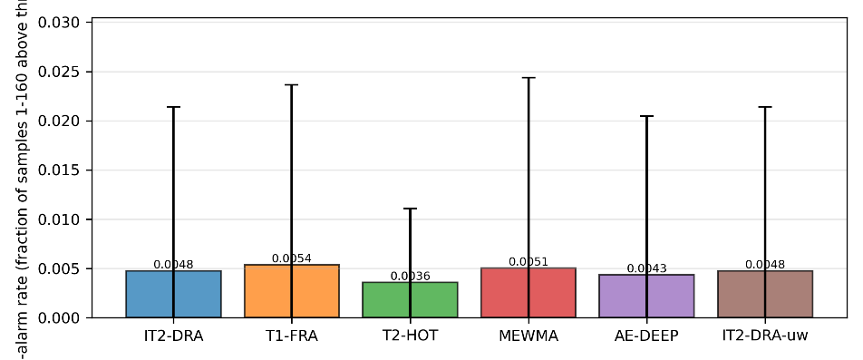
Table 1 reports the aggregate metrics over the 21 faults for all six configurations, and Fig. 1 previews the raw score dynamics for one representative hard fault (fault 4). The proposed IT2-DRA is not competitive with the classical multivariate baselines on this benchmark. Its mean AUC is 0.8099 ± 0.1667, against 0.9183 ± 0.1586 for Hotelling T², 0.9117 ± 0.1553 for MEWMA, and 0.8758 ± 0.1678 for the shallow autoencoder; its mean detection delay is 251.4 samples (median 101) against 98.0 (median 13) for T² and 98.3 (median 15) for MEWMA. The type-1 ablation T1-FRA (0.8105 ± 0.1665, delay 282.3) and the uniform-weight ablation IT2- DRA-uw (0.8122 ± 0.1657) sit within two and a half thousandths of an AUC unit of the proposed method — the changes are small on the AUC scale. Mean false-alarm rates are low for every method (0.0036–0.0054), i.e. roughly 0.6–0.9 false-alarm samples per 160-sample pre-onset window, under the 99th-percentile per-method calibration.
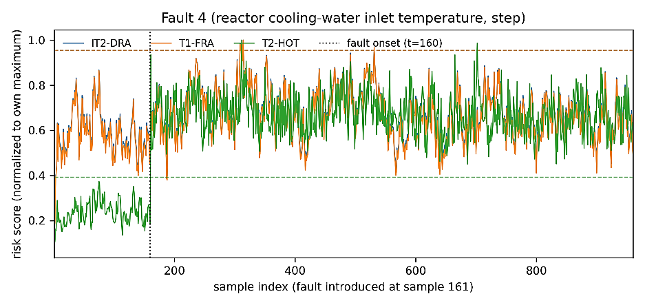
Note (Fig. 1): Dashed lines show method-specific thresholds; the dotted line at index 160 marks the boundary preceding one-based sample 161. Display normalization is not used for fitting or calibration. The multivariate score crosses its threshold promptly, while fuzzy scores remain closer to their thresholds.
Table 1. Aggregate performance over the 21 faults (AUC and false-alarm rate: higher/lower is better; delay in samples after onset, lower is better; censoring at 800 included in means).
This table is shown in the PDF version of the article.
6.2 Global Rank Analysis Friedman and Nemenyi
The reported Friedman tests reject equality on AUC (χ²(4) = 29.288, p = 6.83e−06) and capped delay (χ²(4) = 66.327, p = 1.35e−13), and do not reject equality on per-sample false-alarm rate (p = 0.2483). Table 2 gives mean ranks and CD = 1.3311. On AUC, the rank gap from IT2-DRA exceeds CD for MEWMA, T², and AE-DEEP but not T1-FRA. On delay, T² is best ranked and IT2-DRA fourth. Non-rejection for false alarms is not an equivalence test and cannot certify exactly matched operating points.
Fig. 2 shows the per-fault AUC distributions; Fig. 3 shows the six-method Nemenyi critical-difference diagram on AUC (supplementary analysis with the uniform-weight ablation included, k = 6, CD = 1.6454): The three non-fuzzy baselines form the leading group, and the two fuzzy configurations plus the uniform-weight ablation form a trailing cluster. In the six-method analysis MEWMA is significantly ahead of all three fuzzy configurations, and T² and the autoencoder are significantly ahead of IT2-DRA and T1-FRA (the difference to the uniform-weight variant falls just below CD).
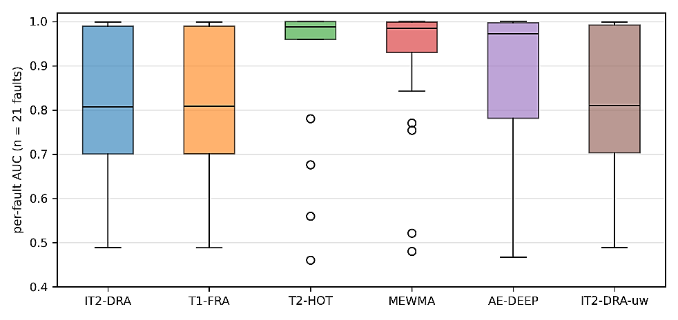
Note (Fig. 2): Boxes show medians and interquartile ranges; whiskers show non-outlier ranges, with more extreme observations plotted separately. The non-fuzzy baselines have higher central AUCs.
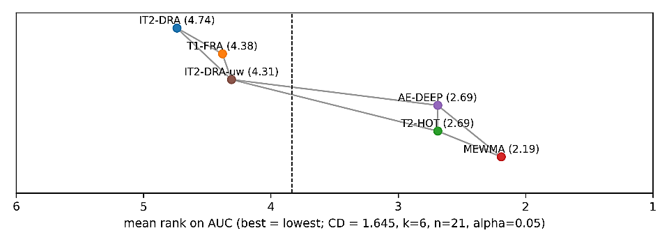
Table 2. Friedman and Nemenyi results across the 21 faults (five primary methods; k = 5, n = 21, α = 0.05).
This table is shown in the PDF version of the article.
6.3 Pairwise Comparisons against IT2-DRA Wilcoxon with Holm Correction
Table 3 reports the two-sided Wilcoxon signed-rank tests of each baseline against IT2-DRA with Holm correction and effect sizes. On AUC, the reported paired tests favor every baseline: MEWMA (p_Holm = 7.90e−04, r = 0.75, mean ΔAUC = +0.1018), AE-DEEP (p_Holm = 0.0015, r = 0.71, +0.0659), T2-HOT (p_Holm = 0.0086, r = 0.60, +0.1084), and — notable for the ablation analysis — even the type-1 fuzzy ablation T1-FRA is significantly different (p_Holm = 0.0303, r = 0.47), albeit with a practically negligible mean advantage of +0.0006 AUC. On detection delay, T2-HOT (p_Holm = 7.63e−06, r = 0.87, mean advantage 153.4 samples), MEWMA (p_Holm = 2.63e−04, r = 0.85, 153.0 samples) and AE-DEEP (p_Holm = 2.63e−04, r = 0.85, 121.1 samples) are all significantly faster, with large effect sizes. The approximate delay comparison against T1-FRA gives p_Holm = 0.317, but is uninformative with one nonzero pair: the two fuzzy configurations have identical delays on 20 of 21 faults, the single exception being fault 4 (Section 7).
Table 3. Two-sided Wilcoxon signed-rank tests against IT2-DRA over the 21 faults (positive AUC difference = baseline higher; positive delay difference = baseline slower; Holm correction over 4 comparisons per metric; r = |Z|/√21).
This table is shown in the PDF version of the article.
6.4 Detection Delay
Fig. 4 compares capped IT2-DRA and MEWMA delays. IT2-DRA is slower on 20 faults, with one tie at 800. Median delays are 13 samples for T², 15 for MEWMA, and 101 for IT2-DRA. IT2-DRA records 800 for faults 9, 14, and 19; T1-FRA also records 800 for fault 4. T² has a recorded delay below 800 for every fault, with maximum 733 on fault 9, while MEWMA records 800 only for fault 14. Fig. 1 illustrates the fault-4 threshold-crossing contrast.
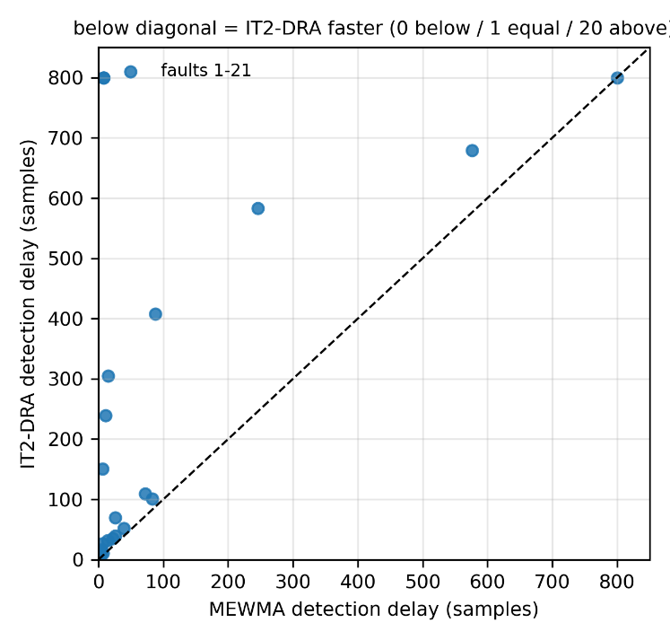
Note (Fig. 4): Twenty points are above the diagonal and one is tied at the censoring value 800. The complete title is “below diagonal = IT2-DRA faster (0 below / 1 equal / 20 above)”; its right edge is truncated in the supplied raster.
6.5 False-Alarm Behavior
Fig. 5 shows mean pre-onset exceedance rates with across-fault standard deviations. The configuration means lie between 0.0036 and 0.0054. The reported Friedman test does not reject equality (p = 0.2483), and no Nemenyi rank gap exceeds CD. These observations support broadly similar measured tail behavior in this campaign, with substantial uncertainty; they do not rule out meaningful false-alarm differences. AUC is threshold-independent, while the delay comparison depends on the chosen quantile and persistence rule.
6.6 Per-Fault Analysis and Failure Mechanism
Table 4 lists the per-fault AUC of all six configurations and Table 5 the per-fault detection delays. Three regimes are clearly separated.
On faults 1, 2, 6, 7, 8, 10, 12, 13, 18, and 20, IT2-DRA has AUC ≥ 0.87; five of these exceed 0.99. Broad deviations can therefore be detected well by the aggregate. This per-fault observation does not imply small gaps for every broad-signature fault.
Faults 3 and 9 produce AUCs near chance for all configurations. IT2-DRA has the highest displayed fault-9 AUC (0.4891), and the uniform-weight ablation has the highest fault-3 AUC (0.5677); neither establishes useful detection. Fault 15 is different: Displayed AUCs range from 0.6761 to 0.7543, so it should not be grouped with near-chance results without qualification.
Table 6 reports the largest persistent mean shift for fault 4 as 7.23 training standard deviations in variable 51, with only one variable exceeding 1σ. Its normalized weight is 0.6/47.6 ≈ 0.0126, so its own instantaneous contribution cannot change the aggregate by more than 1.26 percentage points. The reported total stream means nevertheless differ by 0.049 (0.304 before onset and 0.353 after onset); that difference also reflects changes in other coordinates and their distributions. The squared standardized magnitude 7.23² ≈ 52 is illustrative, not the exact contribution to zᵀ(C+10⁻³I)⁻¹z, which depends on covariance and cross terms. T² attains displayed AUC 1.0000 and delay 3 for this fault, against 0.7434 and 151 for IT2-DRA. Low mean shifts on faults 11, 14, 16, and 19 are consistent with changes beyond location, but mean-shift summaries alone cannot distinguish variance, temporal structure, and correlation changes. The fuzzy score has no explicit cross-variable interaction; its distribution can nonetheless respond to some dependence changes. Fault 21 remains intermediate in the reported comparison.
The aggregate width W_t has reported mean 0.1423 before onset and 0.1272 after onset, increasing on only 8 of 21 faults. For the fixed endpoint widths a = 0.8 and b = 1.2, rU−rL = exp(−z²/(2b²))−exp(−z²/(2a²)); it vanishes at z = 0 and as |z| grows. Differentiation gives its maximum at |z| = √[4a²b² log(b/a)/(b²−a²)] ≈ 1.37. Thus large excursions can shrink this width. Neither these summaries nor the chosen band validate W_t as an onset or confidence indicator.
6.7 Summary of Findings
The reported campaign shows lower mean AUC and longer capped delays for IT2-DRA than for the three non-fuzzy baselines. The interval layer changes mean AUC by less than 0.001 and its delay effect is concentrated in one fault. Uniform weighting changes mean AUC by about 0.0023. Bounded single- *Note: A low mean shift does not establish a covariance-only fault mechanism.
Table 5. Continued.
This table is shown in the PDF version of the article.
Table 6. Selected-fault mean-shift diagnostics in training-standardized units, with corresponding AUCs and capped delays.
This table is shown in the PDF version of the article.
7. Ablation Study
7.1 Interval Type-2 Layer IT2-DRA versus T1-FRA
T1-FRA has mean AUC 0.8105 versus 0.8099 for IT2-DRA. The source reports W = 47, p = 0.0303, and r = 0.47 for the comparison, indicating a small negative AUC change for the interval layer. The reported mean delay decreases from 282.3 to 251.4 entirely because fault 4 changes from the censoring value 800 to 151; other delays are identical. The table’s approximate p = 0.3173 for this one-nonzero-pair delay comparison is not informative: an exact two-sided signed-rank test on one nonzero difference has p = 1. These observations assess endpoint-midpoint aggregation, not Karnik–Mendel inference.
7.2 Criticality Weights IT2-DRA versus Uniform Weights
Uniform weighting raises the reported mean AUC from 0.8099 to 0.8122. The source reports W = 67, p = 0.0958, and r = 0.37. This comparison does not establish equivalence or validate the criticality rationale. Fault 4 has the same recorded delay (151) under both weightings, with AUC 0.7434 versus 0.7575. The available ablation is limited to one alternative weight vector.
8. Discussion
Weighted averaging caps a single coordinate’s contribution and can dilute localized anomalies. The interval width mixture does not remove that cap or introduce explicit joint-coordinate terms. Maximum-type or ordered weighted averaging operators are possible alternatives, but their detection and false-alarm behavior would require new calibration and experiments. The supplied mean-shift diagnostics do not prove that specific faults are purely correlation driven, nor that a different aggregation rule alone would eliminate the observed deficits.
The benchmark aligns with the process-monitoring literature’s emphasis on multivariate structure [8], [9]. It also illustrates why performance of expert-based fuzzy risk prioritization [4], [5] cannot be transferred directly to streaming fault detection. The reported result is evidence about one construction and protocol.
The fuzzy construction offers a simple contribution decomposition and avoids covariance inversion. These are structural properties, not demonstrated distributional robustness or safety guarantees. Percentile calibration supplies a transparent operating rule, but its stability under changed regimes has not been evaluated. An explanatory layer based on individual deviation memberships is a possible application, subject to separate operational validation.
Future studies could compare calibrated extremal aggregation, covariance-aware memberships, and rule-based consequence models. They should retain fault-free fitting and calibration, examine temporal filtering separately, and use replicated or multi-mode data1 [14]. Any extension to safety prioritization should specify severity and decision costs rather than infer risk semantics from anomaly discrimination alone.
9. Threats to Validity and Limitations
Benchmark representativeness: The TE process is a simulation of one plant under one base operating mode, with predominantly step-type faults introduced at a single known sample; real process anomalies are messier, multi-mode, and confounded with operational changes. The streams are short (960 samples, 800 faulty) and 52-dimensional, so per-fault AUC estimates carry non-trivial uncertainty, and the single-fault-per-stream design does not test interacting faults. Our conclusions are therefore about this benchmark family, not about all industrial monitoring tasks; the extended multi-mode release [14] is the appropriate next testbed.
The tested width band, measured/manipulated weights, and weighted mean are fixed choices. Their type-1 and uniform-weight ablations cover only local alternatives. Eq. (5) is midpoint selection after interval aggregation; a rule-based interval type-2 system with centroid type reduction [11], [12] is a different construction and is not evaluated here.
Calibration estimates an extreme quantile from 950 scores in one fault-free record. The persistence rule can reduce isolated threshold exceedances but does not remove quantile-estimation uncertainty. AUC includes warm-up observations and serial dependence. Assigning 800 to undetected streams produces a capped summary, not an estimate of unrestricted mean detection time, and conflates no detection with detection at the final sample. Baselines use different temporal operations, including vector MEWMA versus scalar smoothing. The shallow autoencoder is untuned; no conclusions about state-of-the-art reconstruction methods follow.
The inferential analysis uses 21 heterogeneous fault mechanisms as blocks [15]; these are not independent plant or fault replications. Censoring and tied delays affect rank tests. The single-nonzero-pair type-1 delay comparison requires an exact treatment, and the reported effect-size denominator √21 should not be mistaken for the effective number of nonzero pairs. Raw paired outcomes, zero/tie handling, test options, multiplicity families, and confidence intervals are needed for independent statistical reconstruction. The supplied record does not document preregistration.
10. Conclusion and Future Work
The reported TE campaign favors Hotelling T², MEWMA, and the shallow autoencoder over the tested interval-midpoint fuzzy score on average discrimination and capped delay. IT2-DRA has mean AUC 0.8099 ± 0.1667 and mean capped delay 251.4 samples. Its type-1 counterpart shows a statistically detectable but small AUC advantage, and false-alarm non-rejection does not establish equivalence. Bounded local contributions and absence of explicit joint interactions delimit this construction’s representational capacity; the result does not extend to general interval type-2 fuzzy systems.
The retained per-fault tables and figures provide a concrete comparison for further study. Next steps include calibrated aggregation alternatives, covariance-aware evidence, independent fault replications, and multi-
https://github.com/AIRI-Institute/fddbenchmark mode evaluation [14]. Releasing the implementation and raw outputs is necessary to reproduce the reported comparison and separate algorithmic effects from protocol choices.
Data and Code Availability
The reported experiments use the classic TE challenge files attributed to Downs and Vogel [7] and Chiang et al. [8], obtained from the public mirror https://github.com/qiuruiyu/tennessee-eastman-PCA. The source identifies model_methods.py, run_experiments.py, analyze.py, build_paper.py, results.json, and CSV tables as supporting materials. An accessible study archive or accompanying package is not established by the supplied manuscript. Verification requires the exact input files and hashes, code, environment, per-seed results, thresholds, and statistical outputs.
References
- [1] Zadeh, L. A. (1965). Fuzzy sets. Information and control, 8(3), 338–353. https://doi.org/10.1016/S0019-9958(65)90241-X
- [2] Mendel, J. M., & John, R. I. B. (2002). Type-2 fuzzy sets made simple. IEEE transactions on fuzzy systems, 10(2), 117–127. https://doi.org/10.1109/91.995115
- [3] Mendel, J. M. (2007). Type-2 fuzzy sets and systems: An overview. IEEE computational intelligence magazine, 2(2), 20–29. https://doi.org/10.1109/MCI.2007.357235
- [4] Liou, J. J. H., Guo, B. H. T., Huang, S. W., & Yang, Y. T. (2024). Failure mode and effect analysis using interval type-2 fuzzy and multiple-criteria decision-making methods. Mathematics, 12(24), 1–27. https://doi.org/10.3390/math12243931
- [5] Padash, A., Fattahi, R., & Vahidi, H. (2024). A novel hybrid risk assessment approach under fuzzy environment in steel industry. Engineering applications of artificial intelligence, 133, 108655. https://doi.org/10.1016/j.engappai.2024.108655
- [6] Braniff, A., Akundi, S. S., Liu, Y., Dantas, B., Niknezhad, S. S., Khan, F., … ., & Tian, Y. (2025). Real-time process safety and systems decision-making toward safe and smart chemical manufacturing. Digital chemical engineering, 15, 100227. https://doi.org/10.1016/j.dche.2025.100227
- [7] Downs, J. J., & Vogel, E. F. (1993). A plant-wide industrial process control problem. Computers & chemical engineering, 17(3), 245–255. https://doi.org/10.1016/0098-1354(93)80018-I
- [8] Chiang, L. H., Russell, E. L., & Braatz, R. D. (2012). Fault detection and diagnosis in industrial systems. Springer Science & Business Media. https://doi.org/10.1007/978-1-4471-0347-9
- [9] Russell, E. L., Chiang, L. H., & Braatz, R. D. (2000). Fault detection in industrial processes using canonical variate analysis and dynamic principal component analysis. Chemometrics and intelligent laboratory systems, 51(1), 81–93. https://doi.org/10.1016/S0169-7439(00)00058-7
- [10] Karnik, N. N., Mendel, J. M., & Liang, Q. (1999). Type-2 fuzzy logic systems. IEEE transactions on fuzzy systems, 7(6), 643–658. https://doi.org/10.1109/91.811231
- [11] Liang, Q., & Mendel, J. M. (2000). Interval type-2 fuzzy logic systems: Theory and design. IEEE transactions on fuzzy systems, 8(5), 535–550. https://doi.org/10.1109/91.873577
- [12] Karnik, N. N., & Mendel, J. M. (2001). Centroid of a type-2 fuzzy set. Information sciences, 132(1), 195–220. https://doi.org/10.1016/S0020-0255(01)00069-X
- [13] Tadić, D., & Komatina, N. (2025). A hybrid interval type-2 fuzzy DEMATEL-MABAC approach for strategic failure management in automotive manufacturing. Journal of engineering management and systems engineering (JEMSE), 4(1), 21–38. https://doi.org/10.56578/jemse040102
- [14] Reinartz, C., Kulahci, M., & Ravn, O. (2021). An extended Tennessee Eastman simulation dataset for fault-detection and decision support systems. Computers & chemical engineering, 149, 107281. https://doi.org/10.1016/j.compchemeng.2021.107281
- [15] Demšar, J. (2006). Statistical comparisons of classifiers over multiple data sets. Journal of machine learning research, 7(1), 1–30. https://jmlr.org/papers/v7/demsar06a.html