PM2.5 Forecasting under Controlled Sensor Outages in the Beijing Multi Site Archive

quality, Beijing Multi-Site.

1. Introduction

PM2.5 forecasting combines temporal persistence with spatial information from monitoring stations. Graph-based models encode interactions among stations [1], while attention models can incorporate meteorological and spatial information [2]. Missing observations create a separate design problem: The forecaster must distinguish absent measurements from measured values and decide how to use evidence from the remaining stations. The public Beijing Multi-Site archive records missing values as NA [3], making it a useful setting for studying the effect of additional, controlled outages.

An evaluation based only on isolated missing entries may not describe a station that is unavailable for several consecutive hours. Conversely, an episode-dependent outage model represents a hypothesized association between pollution and missing inputs, rather than an observed account of station failure. Controlled simulation permits the temporal structure and rate of missingness to be varied separately, provided that the realized rates and the information used to construct each mechanism are documented.

Imputation and explicit observation masks offer complementary ways to handle incomplete time series. BRITS learns a bidirectional recurrent imputation model [4], and SAITS uses self-attention [5]. Downstream forecast performance need not follow the ranking of reconstruction errors, so a joint imputation–forecasting design should be compared with inexpensive preprocessing and with a forecaster that simply receives zero-filled inputs. The present experiment examines these alternatives under a shared outage policy.

Three questions guide the comparison: Whether episode-dependent outages increase error relative to independent point dropout at matched rates; whether the joint AirBridge architecture improves on decoupled imputation followed by forecasting; and whether its mask channels, adaptive adjacency and auxiliary reconstruction head improve the reported endpoint. The study includes persistence, hourly climatology, a graph-free temporal model, a distance-graph model, interpolation and recurrent-imputation pipelines, AirBridge and three component ablations. Matching outage conditions across systems and restricting training effort makes the comparison interpretable within this budget, while the reported implementation and training-budget ambiguities remain relevant to replication.

Section 2 relates forecasting and imputation approaches to the study design. Sections 3–5 define the outage models, forecasting systems and evaluation protocol. Section 6 reports the observations, and Sections 7–9 discuss their interpretation, limitations and implications.

2. Related Work

Graph forecasting and geo-sensory attention model spatial and temporal dependence [1], [2]. Recurrent and attention-based imputers address the reconstruction of missing values [4], [5]. These approaches answer different questions: An imputer estimates unavailable inputs, whereas a forecasting architecture maps the available history to a future target. The comparison here evaluates their downstream combination rather than treating accurate reconstruction as sufficient evidence of forecast utility.

Observation masks identify which entries were measured. A zero-filled input alone cannot distinguish a missing entry from a measured zero, and an interpolated input alone does not indicate which values were reconstructed. AirBridge exposes masks directly and includes an auxiliary reconstruction loss. Interpolation and a trained bidirectional recurrent imputer provide decoupled alternatives; their performance is evaluated with the same forecasting endpoint.

The contribution is a controlled comparison on one public multi-station archive. It crosses missingness structure, nominal rate and forecast horizon while retaining inexpensive baselines and component ablations. This design measures the reported systems under the specified perturbations; it does not establish that the simulated outages reproduce maintenance failures or that the tested models span the forecasting literature.

3. Problem Setting and Outage Model

The archive contains twelve stations and 35,064 hourly timestamps from March 2013 through February 2017 [3]. The experiment reports eleven input channels, corresponding to six pollutants and five numeric meteorological variables; the repository also lists categorical wind direction. Each input window contains W = 24 hours, and the targets are PM2.5 concentrations at horizons h ∈ {6, 24}. The experiment reports 1.56% genuine missing entries in the selected channels. Only targets actually observed in the archive are scored. Additional outages affect the input history while leaving observed evaluation targets available. Let m(i,t,c) equal one when a channel is observed and zero when it is unavailable. The three injected missingness rules use nominal fraction ρ:

Point dropout: Pr[m(i,t,c) = 0 due to injection] = ρ, independently across entries. (1)

Station-block outage: Starts occur at rate λ, with block length drawn from an exponential distribution with mean 12 hours; λ is calibrated to the nominal fraction.

Episode-dependent station-block outage: The start intensity is multiplied by 3.0 during city-wide PM2.5 episodes and by 0.4 otherwise, before calibration to the nominal fraction.

Episodes use a training-period 75th-percentile city-wide PM2.5 threshold and reportedly occupy 21.0% of the test period. Calibration uses deterministic seeds and bisection on the realized missing fraction. The denominator must distinguish injected gaps from genuine archive gaps and account for overlap between them. Training augmentation uses window-local versions of the three rules at randomly drawn rates; evaluation uses blocks on a common timeline.

The experiment uses MCAR, MAR and MNAR as labels for point, block and episode-dependent simulation rules. Temporal blocks alone do not define missing at random: A block rule independent of the values may still be MCAR, although its indicators are dependent over time. The episode-dependent rule is MNAR relative to an observation scheme in which the episode-defining pollution values are themselves hidden; otherwise it may be conditionally MAR. The comparisons below therefore emphasize the explicit simulation rules rather than inferring a statistical missingness class from temporal structure alone.

Symmetric Mean Absolute Percentage Error (SMAPE) is reported as a fraction with per-observation value 2|ŷ−y|/(|ŷ|+|y|), bounded between zero and two when the denominator is nonzero. Under this convention, concentrations 5 and 15 give SMAPE = 1.0. A zero-denominator convention is required for implementation. RMSE is measured in µg/m³ and weights large absolute errors more strongly. These endpoints need not select the same system: Table 3 gives Interp+GNN the lowest mean 24-hour SMAPE, but the variant without the imputation head has the lowest reported 24-hour RMSE.

The specified primary setting is the 24-hour forecast under episode-dependent outages at nominal 30% missingness. The analysis also reports aggregates over the outage grid. Because the primary-setting estimate is not separately tabulated, the aggregate comparison should be read as a grid-level analysis rather than a demonstrated test of that primary endpoint.

4. Forecasting Systems under Trial

The study describes compact learned systems with approximately 150,000 parameters, Adam optimization, batch size 64 and a nominal ten-epoch forecasting budget. The distance-graph model uses a Gaussian kernel of haversine distances. Interp+GNN interpolates missing values within each 24-hour input window before forecasting, without using observations beyond the forecast origin. BRITS+GNN is the experiment’s label for a trained bidirectional GRU imputer paired with the forecaster; it is not established as an exact implementation of BRITS [4]. The model labelled GRU is the graph-free temporal comparator, although the architecture specification also describes a shared temporal convolutional backbone.

Learned systems are reported to share optimizer settings and mixed-mechanism augmentation, with two seeds. The recurrent imputer is reported as trained for six epochs, but the description does not resolve whether these epochs supplement or replace forecasting epochs. Equal epoch counts would not imply equal runtime or optimization effort, and the trained imputer adds a separate computational stage. The comparison is therefore a fixed-protocol study with an incompletely specified allocation of effort, rather than a demonstrated equality of total training budgets.

For AirBridge, node i receives the values vᵢ, zero-filled where unavailable, concatenated with binary masks mᵢ. One mask is added per measured channel, giving twenty-two input features for eleven channels. The adaptive adjacency is defined by

B = ReLU(EEᵀ), Aᵢⱼ = Bᵢⱼ / Σₖ Bᵢₖ, E ∈ ℝ^(12×16), for rows with positive sum. (4)

Row normalization makes A row-stochastic on rows with positive total weight. A zero-row fallback must be specified by the implementation. The auxiliary head reconstructs originally observed input entries hidden by augmentation, with the joint objective

L = L_forecast + 0.3 * L_imputation(hidden observed entries). (5)

AirBridge combines mask inputs, adaptive adjacency and an auxiliary reconstruction head with weight 0.3. Ablation A1 removes masks, A2 replaces the adaptive adjacency with the fixed distance graph, and A3 removes the imputation head. Persistence carries forward the last observed station value, with a city-mean fallback when its input history is entirely unavailable. Hourly climatology uses training-period station means for the target hour. Table 1 records the system labels and components as reported.

According to Table 1, Training effort follows the protocol described in Section 5; the recurrent imputer’s epoch allocation requires confirmation.

5. Experimental Protocol

The reported training segment contains the first 24,864 hourly observations starting in March 2013; testing uses January–February 2017, with 1,416 hours and 1,368 forecast origins. Exact timestamps, intervening validation or unused periods, scaler fitting and eligible-origin rules are needed to reconstruct this temporal split. There are nine outage conditions for a given horizon and eighteen across both horizons. Per-setting results average two seeds. The experiment reports Friedman, Nemenyi and paired Wilcoxon analyses with Holm adjustment [6], [7]. The settings reuse the same winter test series and thus are dependent perturbations, not independent datasets.

The UCI repository describes twelve monitoring sites, six pollutants and six meteorological variables, with missing values denoted NA [3]. The present model uses eleven numeric channels. The data are observed environmental records, whereas the additional outage processes are synthetic. Forecast windows, target availability, channel selection and the source of station coordinates must be recorded together for an exact reconstruction.

The experiment reports 1.56% genuine missingness overall, station fractions of 1.0–2.1% and an episode fraction of 21.0% in the test period. These summaries refer to the experiment’s data preparation and require the corresponding counting code. Coordinates enter the fixed graph only. Window-local training corruption and timeline-consistent evaluation blocks expose the learned systems to related, but not identical, perturbation processes.

Rank tests summarize paired system outcomes across outage conditions [6]. The reported p-values remain conditional on the chosen settings and their dependence; two seeds provide limited information about training variability. Table 3 lists component comparisons, and Table 3 gives effect sizes and endpoint-specific orderings. Neither a nonsignificant contrast nor a small point estimate establishes equivalence.

The experiment reports approximately forty minutes on two CPU threads and an evaluation count of one hundred settings. The count’s unit is not defined consistently with the horizon-by-outage design, and the reported claim of twenty learned trainings does not follow directly from eight learned systems with two seeds. A manifest of training runs, outage seeds and evaluation records is required to reconcile these totals.

6. Results

6.1 Effects of Outage Structure and Rate

Fig. 1 shows the 24-hour curves and Fig. 4 their degradation relative to no injected outage. Table 3 places the learned systems between 0.900 and 0.923 mean SMAPE, with aggregate degradation between 0.0038 and 0.0150. Individual cells in Fig. 4 are larger: AirBridge reaches +0.032 under episode-dependent 50% outages. Table 2 reports pooled episode-dependent minus point-dropout differences of +0.0006, +0.0092 and +0.0181 as nominal missingness increases. The modest aggregate differences occur under shared augmentation; without an unaugmented arm, they cannot identify augmentation as the cause.

Table 2. RQ1: Mechanism penalties at matched nominal rates (SMAPE, 24-hour horizon).

This table is shown in the PDF version of the article.

The most affected system in Table 2 changes with rate: Interp+GNN at 10%, BRITS+GNN at 30% and A1 at 50%. The reported curves generally show larger penalties for station blocks at high rates than for independent point dropout. A1’s largest penalty at 50% is compatible with a role for masks under severe episode-dependent missingness, but does not establish that masks have their greatest benefit under that mechanism at every rate.

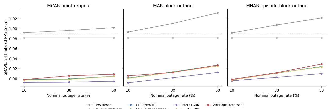
Note (Fig. 1): SMAPE values are fractions; the percent sign in the original axis label is inconsistent with that convention. The series are persistence, hourly climatology, GRU, distance GNN, interpolation+GNN, recurrent-imputer+GNN and AirBridge; the original image’s lower legend is partially cropped.

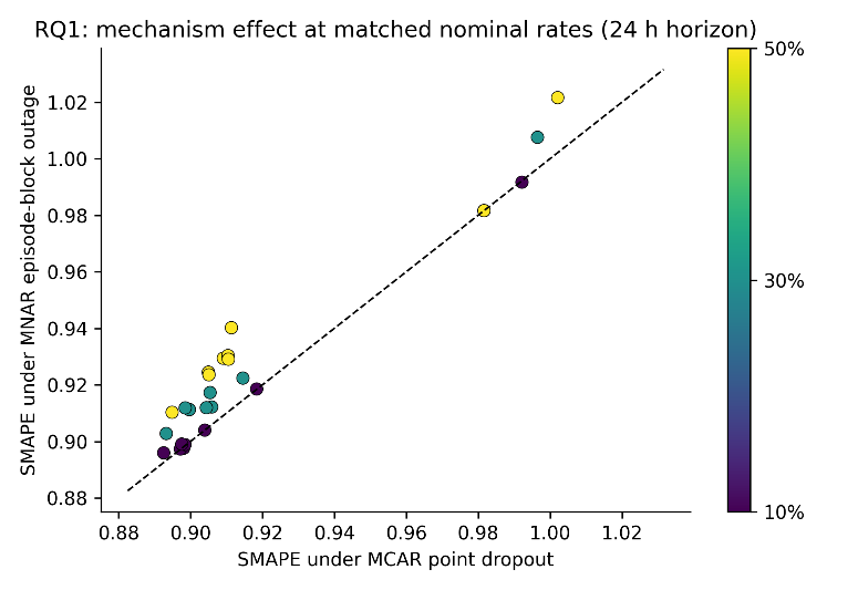
Table 3. Headline aggregates over the outage grid (means over blocks and seeds).

This table is shown in the PDF version of the article.

6.3 RQ3: Which AirBridge Components Earn Their Complexity

The reported AirBridge minus A1 difference is −0.0123 SMAPE, with p = 0.004 in Table 4. AirBridge minus A2 is −0.0018 with p = 0.164, and AirBridge minus A3 is +0.0006 with p = 0.098. Thus masks have the clearest reported component contrast, while the other point estimates are small. These p-values are retained as reported; the dependence of conditions and the adjustment family require verification. Fig. 3’s rank ordering conflicts with some aggregate ordering and with the reported AirBridge rank, so it cannot independently certify these comparisons.

Masks provide an explicit distinction between absent and observed values. This is a plausible explanation for their reported benefit, but a mechanism-specific interaction analysis would be needed to show where that benefit is concentrated. A fixed distance graph and learned adjacency need not span the same family of mixing operators; the small observed contrast does not imply structural equivalence. Similarly, a small auxiliary-head contrast does not prove that reconstruction quality is irrelevant to forecasting.

Table 4. Reported component and pipeline comparisons.

This table is shown in the PDF version of the article.

Note (Table 4): Negative mean ΔSMAPE means A has lower error than B. The source’s p-values and verdict cells are retained; “no effect” is not an equivalence conclusion, and the adjustment status must be reconciled with the text.

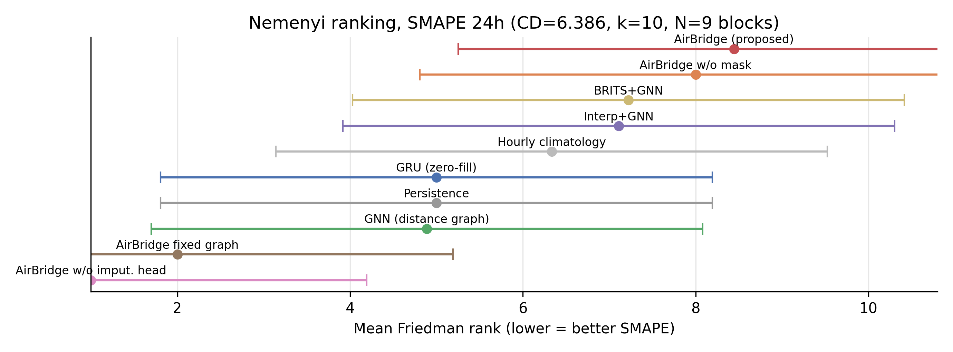
The reported CD is 6.386, approximately 6.39. The conventional Nemenyi formula uses the studentized-range quantile divided by √2; the reported value appears to omit that normalization. The embedded ranks also require verification against per-setting errors. No rank separation is certified here.

6.4 Horizon and Outage Effects

Table 5 and Fig. 5 show a 6-to-24-hour SMAPE increase of 0.216 for Interp+GNN and 0.178 for AirBridge. These horizon differences exceed the pooled mechanism contrasts in Table 2. Outage-rate effects still matter within a fixed horizon, including individual degradation cells around 0.03 at 50% missingness in Fig. 4. The comparison therefore favors evaluating both horizon and outage structure instead of reducing robustness to one aggregate score.

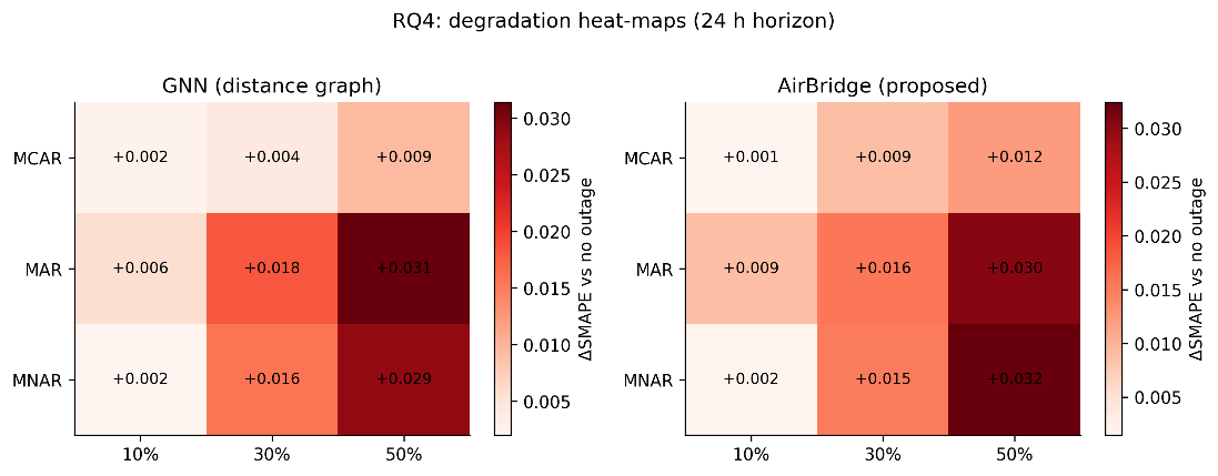
Table 5. Reported horizon effects.

This table is shown in the PDF version of the article.

In Table 5, Each horizon has nine outage conditions; the original caption’s “18 settings” counts both horizons together and must not be interpreted as eighteen independent conditions within a horizon.

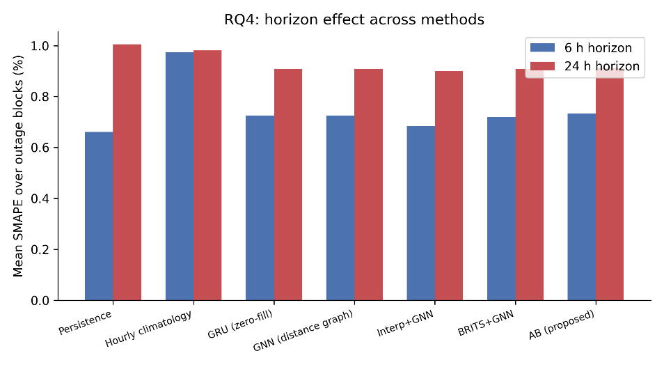
Note: Values are fractions despite the source image’s percent sign. Each horizon contains nine mechanism-by-rate conditions.

7. Discussion

The comparison separates three design choices that are often combined: identifying gaps, estimating their values and modelling spatial dependence. Their reported effects differ within this budget. A compact model with linear interpolation can lead SMAPE without leading RMSE, and a mask-informed model can benefit from masks without benefiting detectably from its other components. The practical lesson is to evaluate each choice against its own inexpensive comparator.

Shared mixed-mechanism augmentation is part of the training protocol, not an independently randomized treatment. A direct test of its contribution would cross augmented and unaugmented training with the same architectures and outage realizations. Likewise, a factorial mask-by-imputation comparison would test whether combining interpolation with explicit masks improves on the configurations actually evaluated here. Interpolation is deterministic within the input window and adds no learned imputation stage. Its reported SMAPE advantage is useful for deciding which baseline to include in a replication. The tested interpolation model has no mask channels in Table 1, so a recipe that combines interpolation and masks is a proposed configuration rather than a result of this campaign.

Evaluation should report the input-window definition, genuine and injected missingness, realized rates, outage duration distribution, target eligibility, augmentation policy and endpoint convention. Persistence and climatology provide horizon-sensitive reference points. The grid should retain per-setting outcomes so that aggregate changes can be traced to particular outage realizations rather than inferred from the overall mean. The episode-dependent rule uses a multiplier of three during high-pollution input hours. Its pooled penalty is approximately 0.02 SMAPE at nominal 50% missingness in this experiment. Stronger coupling, longer outages, an alternative episode definition or correlation with future target episodes could yield different results. None of these variants is established by the present grid.

8. Limitations and Threats to Validity

The data cover one city and twelve stations, with a two-month winter test period. Cross-city transfer and probabilistic endpoints were not evaluated. The injected episode-dependent rule is a modelling choice rather than a mechanism fitted to maintenance logs. Its parameters should not be interpreted as empirically estimated failure probabilities.

Nominal missingness, realized injection and total unavailable fraction may differ when artificial and genuine gaps overlap. Exact calibrator code and observed denominators are needed to verify rate matching. The specification also leaves handling of all-missing channels, interpolation boundaries and persistence fallbacks incomplete.

Approximately 150,000 parameters, a nominal ten forecasting epochs and two seeds restrict the claim to compact systems. Different capacity, tuning, training allocations or seasons could change the ordering. No model was trained without augmentation, and no equivalence margin was specified for small component effects.

The nine conditions per horizon share test hours, targets and trained models. Friedman, Wilcoxon and Nemenyi outputs are therefore exploratory summaries whose conventional independent-block interpretation is limited. The source rank plot conflicts with reported aggregate rankings, and its CD normalization needs correction using the original code. Reported p-values should not be treated as independently verified evidence of general superiority.

The study’s numerical findings require the original data-preparation scripts, exact split timestamps, seeds, model definitions, checkpoints and per-setting outcomes for verification. No accessible replication package is identified in the manuscript. The reported tables and scientific figures give the observational record, but they do not by themselves establish that the claimed programmatic checks or public release occurred.

Station coordinates and their provenance, numeric channel selection, normalization, imputer training effort and the graph-free model definition remain implementation dependencies. Full-year testing, separate outage realizations and more independent training runs would strengthen the assessment of robustness and forecast utility.

9. Conclusion

On the Beijing Multi-Site archive, the reported grid favors interpolation+GNN on 24-hour SMAPE and persistence at six hours. AirBridge’s mask ablation has a larger reported contrast than its graph and auxiliary-head ablations. Episode-dependent outages have a small pooled penalty relative to independent point dropout at low rates and a larger one at nominal 50% missingness. The results support a component-level evaluation with simple baselines, endpoint-specific comparisons and explicit outage specifications. Statistical discrepancies and missing replication evidence limit inferential and operational conclusions; an unaugmented control, verified per-setting analyses and broader temporal validation are the next steps.

References

- [1] Wang, S., Li, Y., Zhang, J., Meng, Q., Meng, L., & Gao, F. (2020). PM2. 5-GNN: A domain knowledge enhanced graph neural network for pm2. 5 forecasting. Proceedings of the 28th international conference on advances in geographic information systems (pp. 163–166). Association for Computing Machinery. https://doi.org/10.1145/3397536.3422208
- [2] Liang, Y., Ke, S., Zhang, J., Yi, X., & Zheng, Y. (2018). Geoman: Multi-level attention networks for geo-sensory time series prediction. [presentation]. Ijcai (pp. 3428–3434). https://doi.org/10.24963/ijcai.2018/476
- [3] Chen, S. (2019). Beijing multi-site air-quality data. UCI machine learning repository, 10, C5RK5G. https://doi.org/10.24432/C5RK5G
- [4] Cao, W., Wang, D., Li, J., Zhou, H., Li, L., & Li, Y. (2018). BRITS: Bidirectional recurrent imputation for time series. Advances in neural information processing systems (Vol. 31). Curran Associates, Inc. https://proceedings.neurips.cc/paper_files/paper/2018/file/734e6bfcd358e25ac1db0a4241b95651-Paper.pdf
- [5] Du, W., Côté, D., & Liu, Y. (2023). SAITS: Self-attention-based imputation for time series. Expert systems with applications, 219, 119619. https://doi.org/10.1016/j.eswa.2023.119619
- [6] Demšar, J. (2006). Statistical comparisons of classifiers over multiple data sets. Journal of machine learning research, 7(1), 1–30. https://jmlr.org/papers/v7/demsar06a.html
- [7] Holm, S. (1979). A simple sequentially rejective multiple test procedure. Scandinavian journal of statistics, 6(2), 65–70. https://www.jstor.org/stable/4615733